

R Tidymodels Parsnip Options Binary Classification
Classification
This lab will exist our first experience with classification models. These models differ from the regression model nosotros saw in the final affiliate by the fact that the response variable is a qualitative variable instead of a continuous variable. This chapter will utilize parsnip for model plumbing fixtures and recipes and workflows to perform the transformations.
The Stock Market Data
We load the tidymodels for modeling functions, ISLR and ISLR2 for data sets, discrim to give us access to discriminant assay models such as LDA and QDA besides every bit the Naive Bayes model and poissonreg for Poisson Regression.
We will exist examining the Smarket data fix for this lab. It contains a number of numeric variables plus a variable called Direction which has the ii labels "Up" and "Down". Earlier nosotros practice on to modeling, permit us take a look at the correlation between the variables.
To look at the correlation, nosotros will utilize the corrr package. The correlate() office volition calculate the correlation matrix between all the variables that it is being fed. We will therefore remove Direction every bit it is not numeric. Then we pass that to rplot() to quickly visualize the correlation matrix. I have too inverse the colours argument to ameliorate run into what is going on.
## ## Correlation method: 'pearson' ## Missing treated using: 'pairwise.complete.obs' rplot ( cor_Smarket, colours = c ( "indianred2", "black", "skyblue1" ) ) ## Don't know how to automatically pick scale for object of type noquote. Defaulting to continuous. 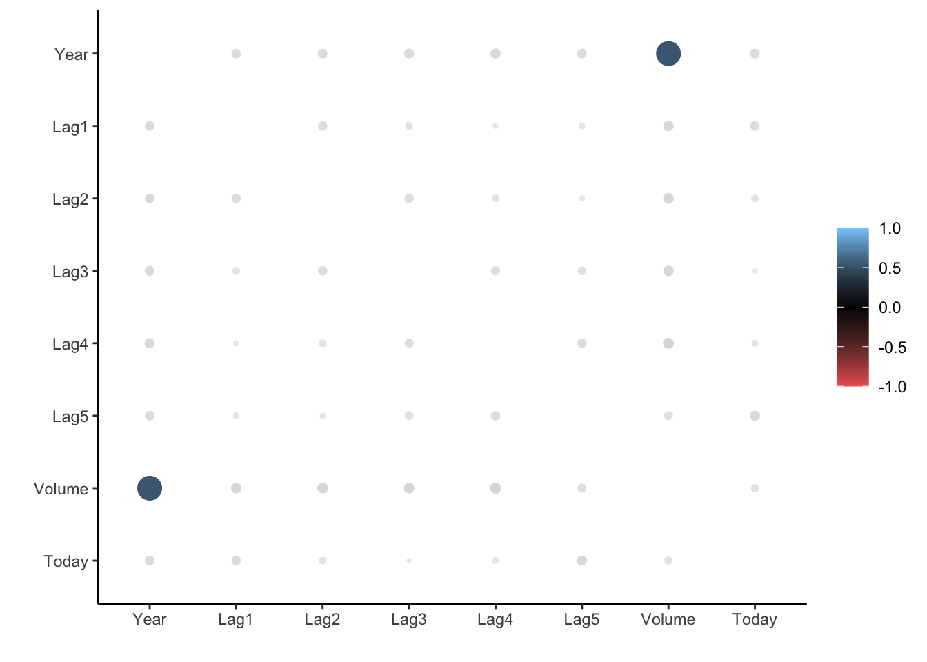
And we see that these variables are more or less uncorrelated with each other. The other pair is Year and Volume that is a niggling correlated.
If you want to create heatmap styled correlation chart you lot can as well create it manually.
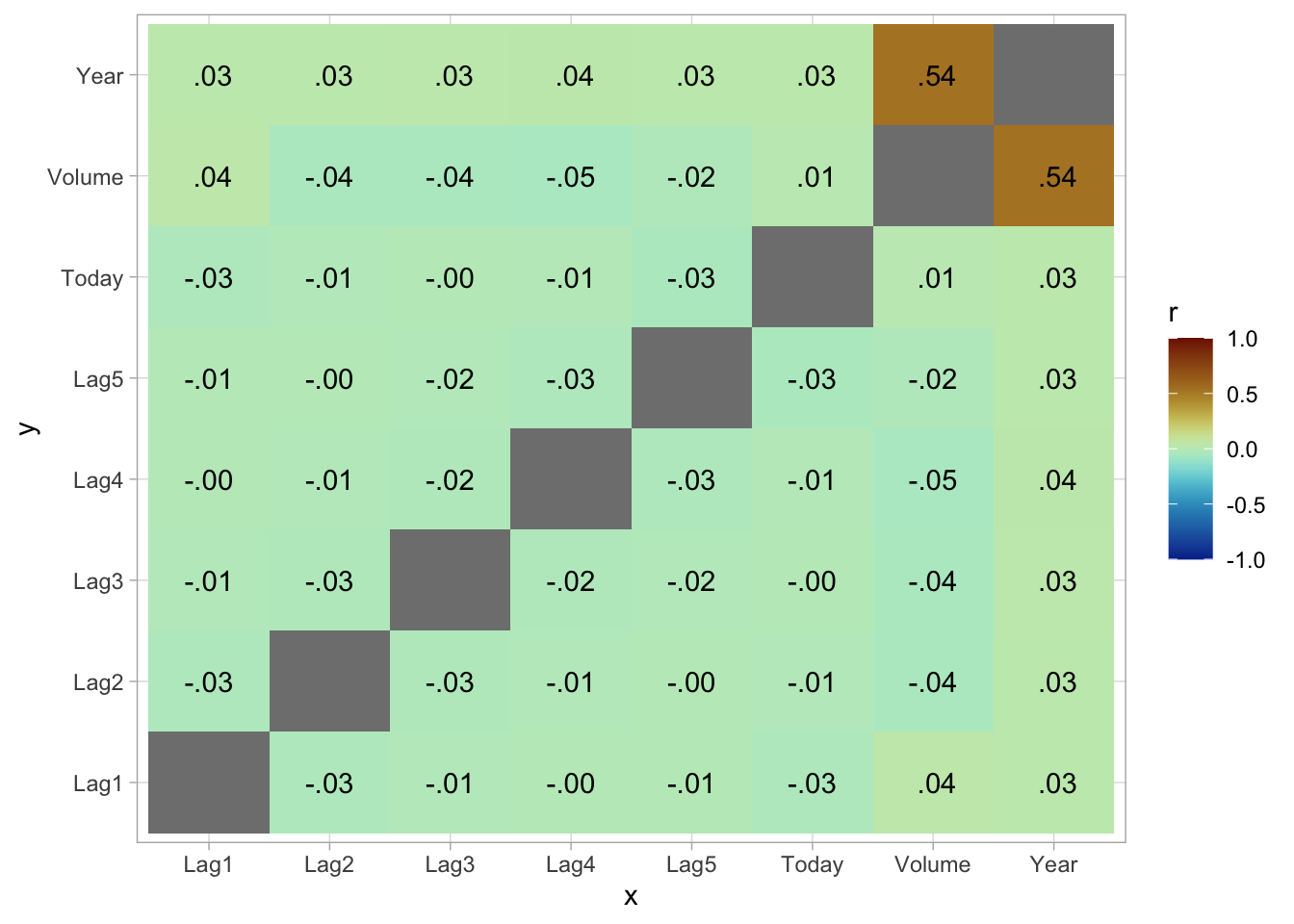
If nosotros plot Yr against Book nosotros see that there is an upwardly trend in Volume with time.
ggplot ( Smarket, aes ( Year, Volume ) ) + geom_jitter (top = 0 ) 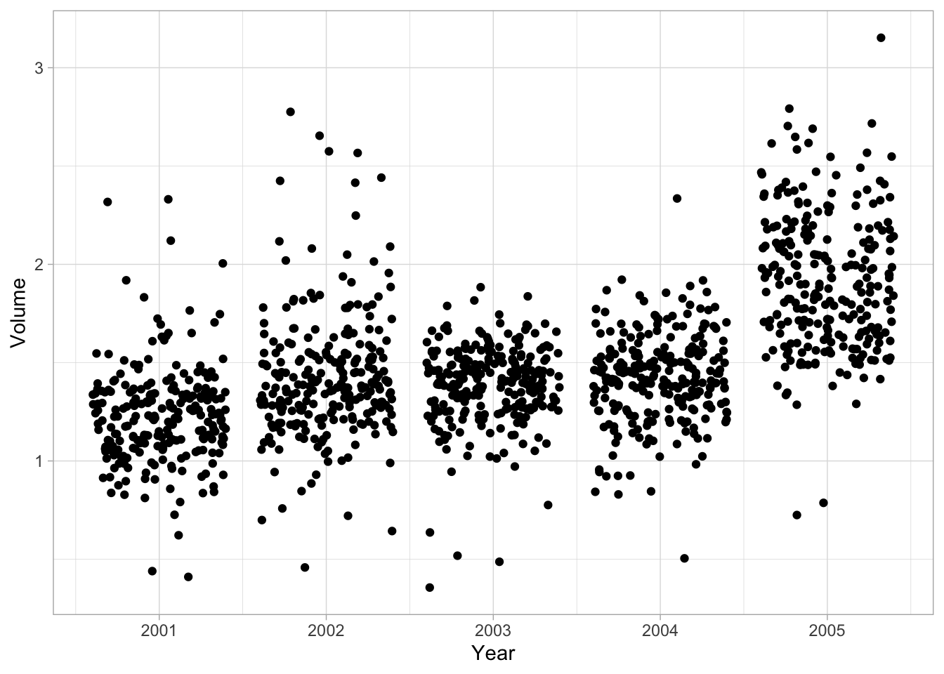
Logistic Regression
At present nosotros will fit a logistic regression model. We will once more use the parsnip package, and nosotros volition utilise logistic_reg() to create a logistic regression model specification.
lr_spec <- logistic_reg ( ) %>% set_engine ( "glm" ) %>% set_mode ( "classification" ) Notice that while I did set the engine and mode, they are just restating the defaults.
Nosotros tin now fit the model like normal. We want to model the Management of the stock market based on the percentage render from the 5 previous days plus the book of shares traded. When plumbing fixtures a classification with parsnip requires that the response variable is a factor. This is the case for the Smarket data fix so nosotros don't need to practice adjustments.
lr_fit <- lr_spec %>% fit ( Direction ~ Lag1 + Lag2 + Lag3 + Lag4 + Lag5 + Book, information = Smarket ) lr_fit ## parsnip model object ## ## Fit time: 7ms ## ## Phone call: stats::glm(formula = Direction ~ Lag1 + Lag2 + Lag3 + Lag4 + ## Lag5 + Volume, family unit = stats::binomial, data = information) ## ## Coefficients: ## (Intercept) Lag1 Lag2 Lag3 Lag4 Lag5 ## -0.126000 -0.073074 -0.042301 0.011085 0.009359 0.010313 ## Volume ## 0.135441 ## ## Degrees of Freedom: 1249 Total (i.east. Null); 1243 Residual ## Null Deviance: 1731 ## Remainder Deviance: 1728 AIC: 1742 this fit is done using the glm() function, and it comes with a very handy summary() method as well.
lr_fit %>% pluck ( "fit" ) %>% summary ( ) ## ## Call: ## stats::glm(formula = Direction ~ Lag1 + Lag2 + Lag3 + Lag4 + ## Lag5 + Volume, family = stats::binomial, data = data) ## ## Deviance Residuals: ## Min 1Q Median 3Q Max ## -one.446 -1.203 1.065 1.145 1.326 ## ## Coefficients: ## Guess Std. Fault z value Pr(>|z|) ## (Intercept) -0.126000 0.240736 -0.523 0.601 ## Lag1 -0.073074 0.050167 -1.457 0.145 ## Lag2 -0.042301 0.050086 -0.845 0.398 ## Lag3 0.011085 0.049939 0.222 0.824 ## Lag4 0.009359 0.049974 0.187 0.851 ## Lag5 0.010313 0.049511 0.208 0.835 ## Volume 0.135441 0.158360 0.855 0.392 ## ## (Dispersion parameter for binomial family taken to be 1) ## ## Aught deviance: 1731.2 on 1249 degrees of freedom ## Residual deviance: 1727.6 on 1243 degrees of freedom ## AIC: 1741.6 ## ## Number of Fisher Scoring iterations: 3 This lets us see a couple of different things such as; parameter estimates, standard errors, p-values, and model fit statistics. nosotros can use the tidy() part to extract some of these model attributes for further assay or presentation.
## # A tibble: 7 × v ## term judge std.mistake statistic p.value ## <chr> <dbl> <dbl> <dbl> <dbl> ## 1 (Intercept) -0.126 0.241 -0.523 0.601 ## 2 Lag1 -0.0731 0.0502 -1.46 0.145 ## 3 Lag2 -0.0423 0.0501 -0.845 0.398 ## four Lag3 0.0111 0.0499 0.222 0.824 ## v Lag4 0.00936 0.0500 0.187 0.851 ## half dozen Lag5 0.0103 0.0495 0.208 0.835 ## 7 Book 0.135 0.158 0.855 0.392 Predictions are done much the same mode. Here we use the model to predict on the data it was trained on.
predict ( lr_fit, new_data = Smarket ) ## # A tibble: 1,250 × 1 ## .pred_class ## <fct> ## 1 Upward ## 2 Down ## three Down ## four Up ## 5 Up ## 6 Up ## seven Down ## eight Up ## 9 Up ## 10 Down ## # … with 1,240 more than rows The result is a tibble with a single cavalcade .pred_class which will be a factor variable of the same labels as the original training data set.
We tin can also get dorsum probability predictions, by specifying type = "prob".
predict ( lr_fit, new_data = Smarket, type = "prob" ) ## # A tibble: 1,250 × 2 ## .pred_Down .pred_Up ## <dbl> <dbl> ## one 0.493 0.507 ## 2 0.519 0.481 ## 3 0.519 0.481 ## 4 0.485 0.515 ## 5 0.489 0.511 ## 6 0.493 0.507 ## 7 0.507 0.493 ## 8 0.491 0.509 ## ix 0.482 0.518 ## 10 0.511 0.489 ## # … with 1,240 more rows note that nosotros get back a cavalcade for each of the classes. This is a little reductive since we could easily summate the inverse, but once we get to multi-classification models information technology becomes quite handy.
Using broaden() nosotros tin add together the predictions to the data.frame and so apply that to wait at model functioning metrics. before we calculate the metrics directly, I observe information technology useful to look at the confusion matrix. This will bear witness you how well your predictive model is performing past given a tabular array of predicted values against the true value.
augment ( lr_fit, new_data = Smarket ) %>% conf_mat (truth = Direction, guess = .pred_class ) ## Truth ## Prediction Downwards Up ## Down 145 141 ## Upwards 457 507 A good performing model would ideally have high numbers along the diagonal (up-left to downwards-right) with modest numbers on the off-diagonal. Nosotros see here that the model isn't nifty, every bit information technology tends to predict "Downward" as "Upwardly" more oft than it should.
if yous want a more visual representation of the confusion matrix yous tin can pipe the event of conf_mat() into autoplot() to generate a ggplot2 chart.
augment ( lr_fit, new_data = Smarket ) %>% conf_mat (truth = Direction, estimate = .pred_class ) %>% autoplot (type = "heatmap" ) 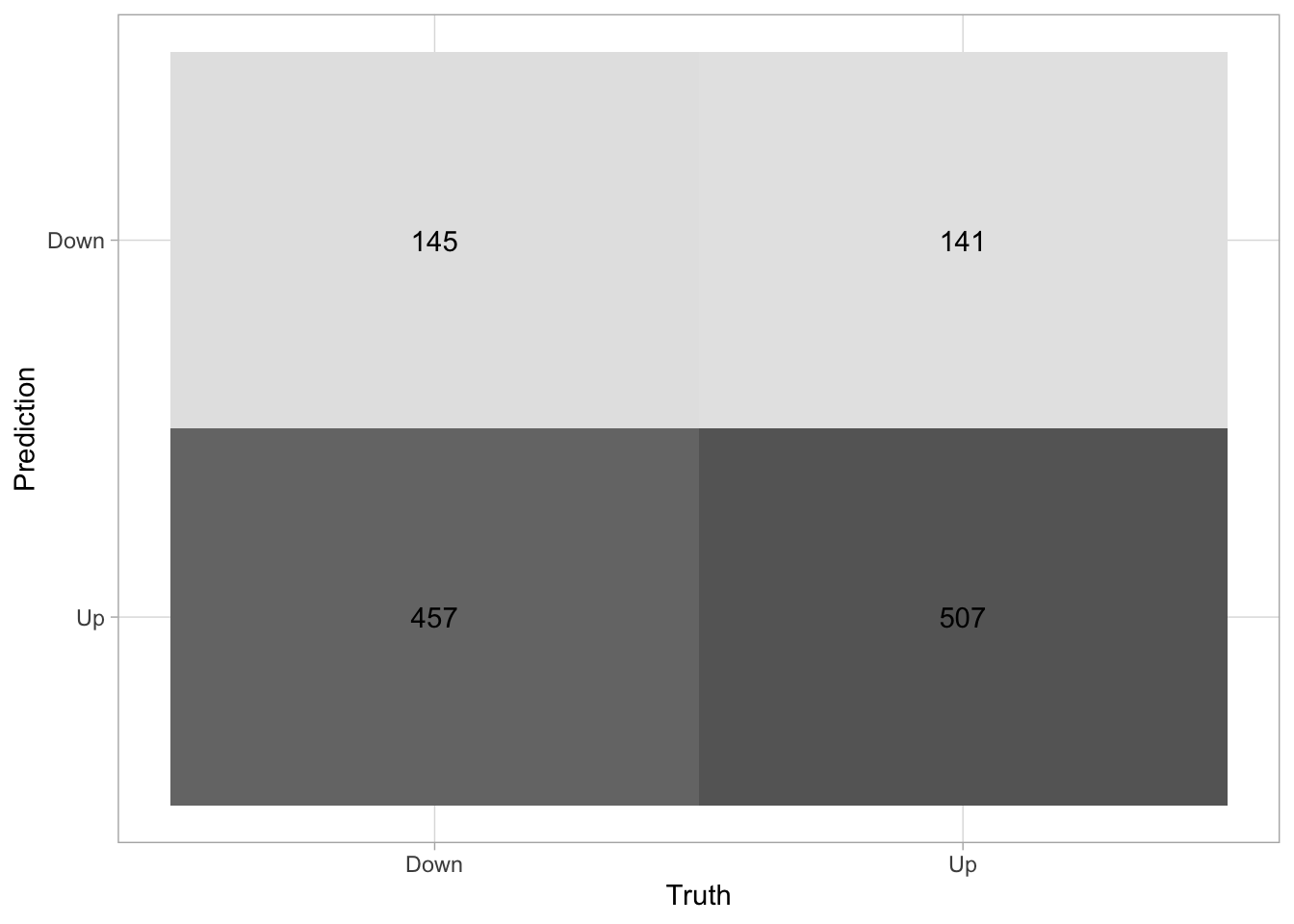
We tin can also summate various performance metrics. One of the nigh common metrics is accuracy, which is how often the model predicted correctly as a percentage.
augment ( lr_fit, new_data = Smarket ) %>% accuracy (truth = Direction, estimate = .pred_class ) ## # A tibble: 1 × 3 ## .metric .estimator .judge ## <chr> <chr> <dbl> ## ane accuracy binary 0.522 and we encounter that the accuracy isn't great either which is obvious already looking at the defoliation matrix.
We only fit a model and evaluated information technology on the same data. This doesn't give us that much data near the model performance. Let us instead divide upwardly the data, train it on some of it and so evaluate information technology on the other part of the data. Since we are working with some data that has a time component, it is natural to fit the model using the commencement year'southward worth of information and evaluate it on the final year. This would more closely match how such a model would be used in existent life.
Smarket_train <- Smarket %>% filter ( Twelvemonth != 2005 ) Smarket_test <- Smarket %>% filter ( Twelvemonth == 2005 ) Now that nosotros have split the data into Smarket_train and Smarket_test we can fit a logistic regression model to Smarket_train and evaluate it on Smarket_test to see how well the model generalizes.
lr_fit2 <- lr_spec %>% fit ( Management ~ Lag1 + Lag2 + Lag3 + Lag4 + Lag5 + Volume, data = Smarket_train ) And we will evaluate on the testing data ready.
augment ( lr_fit2, new_data = Smarket_test ) %>% conf_mat (truth = Direction, approximate = .pred_class ) ## Truth ## Prediction Down Upward ## Down 77 97 ## Up 34 44 augment ( lr_fit2, new_data = Smarket_test ) %>% accurateness (truth = Direction, estimate = .pred_class ) ## # A tibble: 1 × 3 ## .metric .figurer .judge ## <chr> <chr> <dbl> ## 1 accuracy binary 0.480 We see that this model is not more than likely to predict "Down" rather than "Up". Besides, annotation how the model performs worse than the concluding model. This is expected since we are evaluating on new data.
We recall that the logistic regression model had underwhelming p-values. Let usa see what happens if we remove some of the variables that appear not to be helpful we might reach a more predictive model since the variables that exercise non take a relationship with the response will cause an increment in variance without a decrease in bias.
lr_fit3 <- lr_spec %>% fit ( Direction ~ Lag1 + Lag2, data = Smarket_train ) augment ( lr_fit3, new_data = Smarket_test ) %>% conf_mat (truth = Direction, gauge = .pred_class ) ## Truth ## Prediction Downwards Upwards ## Down 35 35 ## Up 76 106 augment ( lr_fit3, new_data = Smarket_test ) %>% accurateness (truth = Direction, gauge = .pred_class ) ## # A tibble: i × iii ## .metric .estimator .gauge ## <chr> <chr> <dbl> ## one accuracy binary 0.560 And we see an increment in performance. The model is still not perfect just information technology is starting to perform amend.
Suppose that we want to predict the returns associated with detail values of Lag1 and Lag2. In detail, nosotros want to predict Direction on a mean solar day when Lag1 and Lag2 equal 1.ii and 1.one, respectively, and on a day when they equal 1.five and −0.eight.
For this we start by creating a tibble corresponding to the scenarios we want to predict for
Smarket_new <- tibble ( Lag1 = c ( ane.2, 1.5 ), Lag2 = c ( one.i, - 0.viii ) ) And and then we volition use predict()
predict ( lr_fit3, new_data = Smarket_new, blazon = "prob" ) ## # A tibble: 2 × ii ## .pred_Down .pred_Up ## <dbl> <dbl> ## 1 0.521 0.479 ## 2 0.504 0.496 Linear Discriminant Analysis
Now we will perform LDA on the Smarket data. We will use the discrim_linear() function to create a LDA specification. We will keep to use 2 predictors for easy comparison.
lda_spec <- discrim_linear ( ) %>% set_mode ( "nomenclature" ) %>% set_engine ( "MASS" ) lda_fit <- lda_spec %>% fit ( Direction ~ Lag1 + Lag2, information = Smarket_train ) lda_fit ## parsnip model object ## ## Fit time: 5ms ## Call: ## lda(Management ~ Lag1 + Lag2, data = information) ## ## Prior probabilities of groups: ## Downwards Up ## 0.491984 0.508016 ## ## Group means: ## Lag1 Lag2 ## Down 0.04279022 0.03389409 ## Upwardly -0.03954635 -0.03132544 ## ## Coefficients of linear discriminants: ## LD1 ## Lag1 -0.6420190 ## Lag2 -0.5135293 Ane of the things to wait for in the LDA output is the group means. We see that there is a slight deviation betwixt the ways of the ii groups. These suggest that at that place is a tendency for the previous two days' returns to exist negative on days when the market increases, and a tendency for the previous day' returns to be positive on days when the market declines.
Predictions are done merely the same as with logistic regression
predict ( lda_fit, new_data = Smarket_test ) ## # A tibble: 252 × 1 ## .pred_class ## <fct> ## 1 Up ## ii Up ## 3 Up ## iv Upward ## 5 Upwardly ## 6 Up ## 7 Up ## 8 Upwardly ## 9 Upward ## x Up ## # … with 242 more rows predict ( lda_fit, new_data = Smarket_test, type = "prob" ) ## # A tibble: 252 × two ## .pred_Down .pred_Up ## <dbl> <dbl> ## 1 0.490 0.510 ## 2 0.479 0.521 ## 3 0.467 0.533 ## 4 0.474 0.526 ## 5 0.493 0.507 ## 6 0.494 0.506 ## 7 0.495 0.505 ## 8 0.487 0.513 ## 9 0.491 0.509 ## 10 0.484 0.516 ## # … with 242 more rows And we can take a look at the operation.
augment ( lda_fit, new_data = Smarket_test ) %>% conf_mat (truth = Direction, estimate = .pred_class ) ## Truth ## Prediction Down Upward ## Downward 35 35 ## Up 76 106 augment ( lda_fit, new_data = Smarket_test ) %>% accuracy (truth = Direction, judge = .pred_class ) ## # A tibble: 1 × 3 ## .metric .figurer .estimate ## <chr> <chr> <dbl> ## one accuracy binary 0.560 And we see no markedly deviation functioning between this model and the logistic regression model.
Quadratic Discriminant Analysis
We will at present fit a QDA model. The discrim_quad() office is used hither.
Once nosotros have the model specification fitting the model is merely like before.
qda_spec <- discrim_quad ( ) %>% set_mode ( "classification" ) %>% set_engine ( "MASS" ) qda_fit <- qda_spec %>% fit ( Management ~ Lag1 + Lag2, information = Smarket_train ) augment ( qda_fit, new_data = Smarket_test ) %>% conf_mat (truth = Direction, judge = .pred_class ) ## Truth ## Prediction Downward Up ## Down 30 20 ## Up 81 121 broaden ( qda_fit, new_data = Smarket_test ) %>% accuracy (truth = Direction, estimate = .pred_class ) ## # A tibble: 1 × 3 ## .metric .estimator .estimate ## <chr> <chr> <dbl> ## 1 accuracy binary 0.599 And we are seeing another increase in accuracy. However this model nevertheless rarely predicts "Downwardly'. This make it appear that the quadratic form assumed by QDA captures the relationship more clearly.
Naive Bayes
We will now fit a Naive Bayes model to the Smarket information. For this, we volition be using the naive_bayes() function to create the specification and also ready the usekernel argument to Faux. This ways that nosotros are assuming that the predictors Lag1 and Lag2 are drawn from Gaussian distributions.
Once the model is specified, the plumbing equipment process is exactly similar before
nb_spec <- naive_Bayes ( ) %>% set_mode ( "nomenclature" ) %>% set_engine ( "klaR" ) %>% set_args (usekernel = False ) nb_fit <- nb_spec %>% fit ( Direction ~ Lag1 + Lag2, data = Smarket_train ) In one case the model is fit, we can create the confusion matrix based on the testing data and likewise assess the model accuracy.
augment ( nb_fit, new_data = Smarket_test ) %>% conf_mat (truth = Direction, estimate = .pred_class ) ## Truth ## Prediction Down Up ## Downwards 28 twenty ## Upwardly 83 121 augment ( nb_fit, new_data = Smarket_test ) %>% accuracy (truth = Direction, judge = .pred_class ) ## # A tibble: 1 × iii ## .metric .estimator .estimate ## <chr> <chr> <dbl> ## 1 accuracy binary 0.591 The accuracy of the Naive Bayes is very similar to that of the QDA model. This seems reasonable since the below scatter plot shows that there is no apparent human relationship betwixt Lag1 vs Lag2 and thus the Naive Bayes' assumption of independently distributed predictors is not unreasonable.
ggplot ( Smarket, aes ( Lag1, Lag2 ) ) + geom_point (alpha = 0.1, size = 2 ) + geom_smooth (method = "lm", se = FALSE ) + labs (title = "No apparent correlation between Lag1 and Lag2" ) ## `geom_smooth()` using formula 'y ~ ten' 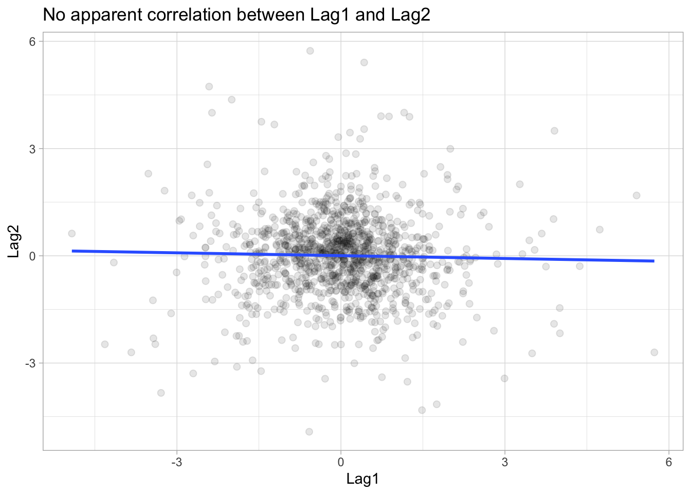
K-Nearest Neighbors
Lastly permit us have a look at a K-Nearest Neighbors model. This is the first model we accept looked at that has a hyperparameter we demand to specify. I take set it to 3 with neighbors = 3. Plumbing fixtures is done like normal.
knn_spec <- nearest_neighbor (neighbors = 3 ) %>% set_mode ( "nomenclature" ) %>% set_engine ( "kknn" ) knn_fit <- knn_spec %>% fit ( Management ~ Lag1 + Lag2, data = Smarket_train ) knn_fit ## parsnip model object ## ## Fit time: 36ms ## ## Call: ## kknn::train.kknn(formula = Management ~ Lag1 + Lag2, data = data, ks = min_rows(3, data, v)) ## ## Type of response variable: nominal ## Minimal misclassification: 0.492986 ## All-time kernel: optimal ## Best chiliad: three And evaluation is washed the same way
augment ( knn_fit, new_data = Smarket_test ) %>% conf_mat (truth = Direction, guess = .pred_class ) ## Truth ## Prediction Downwardly Upwardly ## Down 43 58 ## Up 68 83 augment ( knn_fit, new_data = Smarket_test ) %>% accuracy (truth = Direction, gauge = .pred_class ) ## # A tibble: 1 × iii ## .metric .estimator .estimate ## <chr> <chr> <dbl> ## 1 accuracy binary 0.5 Information technology appears that this model is not performing that well.
Nosotros volition try using a K-nearest neighbors model in an application to caravan insurance data. This information set includes 85 predictors that measure demographic characteristics for 5822 individuals. The response variable is Purchase, which indicates whether or not a given individual purchases a caravan insurance policy. In this data set, only 6% of people purchased caravan insurance.
Nosotros want to build a predictive model that uses the demographic characteristics to predict whether an individual is going to buy a caravan insurance. Earlier we go along, we split the information set into a training information fix and testing information set. (This is a not the proper mode this should be done. See side by side chapter for the right way.)
Caravan_test <- Caravan [ seq_len ( 1000 ), ] Caravan_train <- Caravan [ - seq_len ( 1000 ), ] Since we are using a Grand-nearest neighbour model, it is importance that the variables are centered and scaled to make sure that the variables have a uniform influence. We can reach this transformation with step_normalize(), which does centering and scaling in one go.
rec_spec <- recipe ( Purchase ~ ., data = Caravan_train ) %>% step_normalize ( all_numeric_predictors ( ) ) Nosotros will exist trying different values of K to see how the number of neighbors affect the model performance. A workflow object is created, with just the recipe added.
Caravan_wf <- workflow ( ) %>% add_recipe ( rec_spec ) Next nosotros create a general KNN model specification.
knn_spec <- nearest_neighbor ( ) %>% set_mode ( "classification" ) %>% set_engine ( "kknn" ) We tin can so use this model specification along with Caravan_wf to create three total workflow objects for K = 1,three,5.
knn1_wf <- Caravan_wf %>% add_model ( knn_spec %>% set_args (neighbors = 1 ) ) knn3_wf <- Caravan_wf %>% add_model ( knn_spec %>% set_args (neighbors = 3 ) ) knn5_wf <- Caravan_wf %>% add_model ( knn_spec %>% set_args (neighbors = 5 ) ) With all these workflow specification nosotros can fit all the models one by ane.
knn1_fit <- fit ( knn1_wf, data = Caravan_train ) knn3_fit <- fit ( knn3_wf, data = Caravan_train ) knn5_fit <- fit ( knn5_wf, data = Caravan_train ) And we can calculate all the confusion matrices.
broaden ( knn1_fit, new_data = Caravan_test ) %>% conf_mat (truth = Purchase, approximate = .pred_class ) ## Truth ## Prediction No Yes ## No 874 50 ## Yep 67 9 augment ( knn3_fit, new_data = Caravan_test ) %>% conf_mat (truth = Buy, estimate = .pred_class ) ## Truth ## Prediction No Yes ## No 875 50 ## Yes 66 ix augment ( knn5_fit, new_data = Caravan_test ) %>% conf_mat (truth = Purchase, estimate = .pred_class ) ## Truth ## Prediction No Yes ## No 874 50 ## Yes 67 nine And it appears that the model performance doesn't alter much when changing from 1 to 5.
Poisson Regression
So far we take been using the Smarket data fix to predict the stock price movement. We will now shift to a new information set, Bikeshare, and look at the number of cycle rentals per hour in Washington, D.C.
The variable of interest, number of bike rentals per hour tin accept on non-negative integer values. This makes Poisson Regression a suitable candidate to model the same.
We get-go with specifying the model using the poisson_reg() function.
pois_spec <- poisson_reg ( ) %>% set_mode ( "regression" ) %>% set_engine ( "glm" ) Hither we volition be predicting bikers using the following predictors:
-
mnth- month of the year, coded as a factor -
hr- 60 minutes of the day, coded every bit a factor from 0 to 23 -
workingday- Is information technology a workday? Already coded as a dummy variable with Yes = 1, No = 0 -
temp- normalized temperature in Celsius -
weathersit- weather condition condition, again coded as a cistron with the following levels:- clear
- cloudy/misty
- light rain/snow
- heavy rain/snowfall
As nosotros can encounter, apart from temp all other predictors are chiselled in nature. Thus, we volition first create a recipe to convert these into dummy variables and and so packet the model spec and recipe using a workflow.
pois_rec_spec <- recipe ( bikers ~ mnth + 60 minutes + workingday + temp + weathersit, data = Bikeshare ) %>% step_dummy ( all_nominal_predictors ( ) ) pois_wf <- workflow ( ) %>% add_recipe ( pois_rec_spec ) %>% add_model ( pois_spec ) With the workflow in place, we follow the same pattern to fit the model and look at the predictions.
pois_fit <- pois_wf %>% fit (data = Bikeshare ) broaden ( pois_fit, new_data = Bikeshare, type.predict = "response" ) %>% ggplot ( aes ( bikers, .pred ) ) + geom_point (alpha = 0.i ) + geom_abline (slope = 1, size = ane, colour = "grey40" ) + labs (title = "Predicting the number of bikers per hour using Poission Regression", x = "Bodily", y = "Predicted" ) 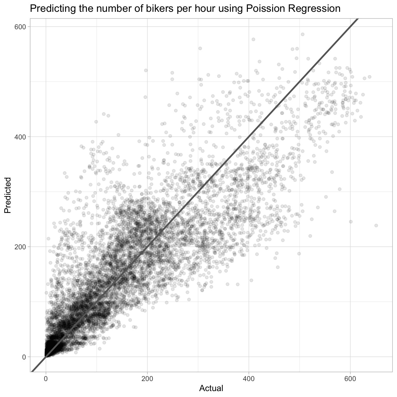
Nosotros tin can also wait at the model coefficients to get a feel for the working of the model and comparison it with our own understanding.
Looking at the coefficients corresponding to the mnth variable, we note that information technology is lower in the wintertime months and higher in the summer months. This seems logical equally nosotros would expect the number of bike rentals to exist college during summertime.
pois_fit_coef_mnths <- tidy ( pois_fit ) %>% filter ( grepl ( "^mnth", term ) ) %>% mutate ( term = stringr :: str_replace ( term, "mnth_", "" ), term = forcats :: fct_inorder ( term ) ) pois_fit_coef_mnths %>% ggplot ( aes ( term, judge ) ) + geom_line (group = 1 ) + geom_point (shape = 21, size = 3, stroke = ane.five, make full = "black", color = "white" ) + labs (championship = "Coefficient value from Poission Regression", x = "Calendar month", y = "Coefficient" ) 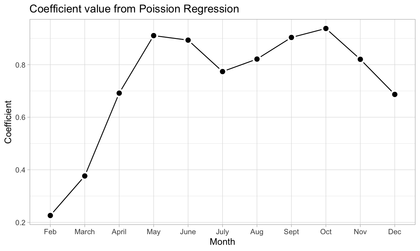
Nosotros tin similarly also look at the coefficients corresponding to the hr variable. Here the peaks occur at eight:00 AM and 5:00 PM, i.eastward. during normal office outset and end times.
pois_fit_coef_hr <- tidy ( pois_fit ) %>% filter ( grepl ( "^hr", term ) ) %>% mutate ( term = stringr :: str_replace ( term, "hr_X", "" ), term = forcats :: fct_inorder ( term ) ) pois_fit_coef_hr %>% ggplot ( aes ( term, estimate ) ) + geom_line (group = 1 ) + geom_point (shape = 21, size = three, stroke = 1.5, make full = "black", colour = "white" ) + labs (title = "Coefficient value from Poission Regression", 10 = "Month", y = "Coefficient" ) 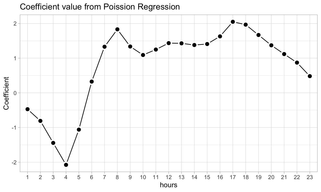

R Tidymodels Parsnip Options Binary Classification,
Source: https://emilhvitfeldt.github.io/ISLR-tidymodels-labs/classification.html
Posted by: jacksonnotilen.blogspot.com
0 Response to "R Tidymodels Parsnip Options Binary Classification"
Post a Comment